Mehrere Kompetenzbereiche: Schleifen
loop_example.RmdData preperation
The data we are using in this example is nexted into multiple competence areas. Let’s take a look:
str(dispar)
#> List of 5
#>  $ hoeren:List of 4
#>   ..$ plain      :'data.frame':  2331 obs. of  17 variables:
#>   .. ..$ label1       : chr [1:2331] "trend (2015 - 2009) for BadenWuerttemberg_maennlich" "trend (2015 - 2009) for crossDiff (BadenWuerttemberg_maennlich - BadenWuerttemberg_total) " "trend (2015 - 2009) of groupDiff (maennlich - weiblich) in TR_BUNDESLAND=BadenWuerttemberg" "trend (2015 - 2009) for BadenWuerttemberg_total" ...
#>   .. ..$ label2       : chr [1:2331] "year=2015 - year=2009: TR_BUNDESLAND=BadenWuerttemberg, Kgender=maennlich" "[year=2015: (TR_BUNDESLAND=BadenWuerttemberg, Kgender=maennlich)] - [year=2009: (TR_BUNDESLAND=BadenWuerttember"| __truncated__ "[year=2015: (TR_BUNDESLAND=BadenWuerttemberg, Kgender=maennlich) - (TR_BUNDESLAND=BadenWuerttemberg, Kgender=we"| __truncated__ "year=2015 - year=2009: TR_BUNDESLAND=BadenWuerttemberg, Kgender=total" ...
#>   .. ..$ unit_1       : chr [1:2331] "group_31" "comp_757" "comp_154" "group_202" ...
#>   .. ..$ unit_2       : chr [1:2331] "group_225" "comp_1373" "comp_307" "group_339" ...
#>   .. ..$ depVar       : chr [1:2331] "bista" "bista" "bista" "bista" ...
#>   .. ..$ modus        : chr [1:2331] "JK2.mean__BIFIEsurvey" "JK2.mean__BIFIEsurvey" "JK2.mean__BIFIEsurvey" "JK2.mean__BIFIEsurvey" ...
#>   .. ..$ parameter    : chr [1:2331] "mean" "mean" "mean" "mean" ...
#>   .. ..$ comparison   : chr [1:2331] "trend" "trend_crossDiff" "trend_groupDiff" "trend" ...
#>   .. ..$ TR_BUNDESLAND: chr [1:2331] "BadenWuerttemberg" "BadenWuerttemberg" "BadenWuerttemberg" "BadenWuerttemberg" ...
#>   .. ..$ Kgender      : chr [1:2331] "maennlich" "maennlich - total" "maennlich - weiblich" "total" ...
#>   .. ..$ year         : chr [1:2331] "2015 - 2009" "2015 - 2009" "2015 - 2009" "2015 - 2009" ...
#>   .. ..$ id           : chr [1:2331] "comp_32" "comp_758" "comp_155" "comp_203" ...
#>   .. ..$ kb           : chr [1:2331] "hoeren" "hoeren" "hoeren" "hoeren" ...
#>   .. ..$ est          : num [1:2331] -40.74 -6.47 12.97 -34.27 -27.77 ...
#>   .. ..$ se           : num [1:2331] 7.66 9.42 8.18 6.15 6.71 ...
#>   .. ..$ p            : num [1:2331] 0 0.492 0.113 0 0 0.453 0.004 0 0.605 0.001 ...
#>   .. ..$ es           : num [1:2331] -0.395 NA NA -0.336 -0.282 NA NA NA NA NA ...
#>   ..$ comparisons:'data.frame':  1719 obs. of  4 variables:
#>   .. ..$ id        : chr [1:1719] "comp_32" "comp_758" "comp_155" "comp_203" ...
#>   .. ..$ unit_1    : chr [1:1719] "group_31" "comp_757" "comp_154" "group_202" ...
#>   .. ..$ unit_2    : chr [1:1719] "group_225" "comp_1373" "comp_307" "group_339" ...
#>   .. ..$ comparison: chr [1:1719] "trend" "trend_crossDiff" "trend_groupDiff" "trend" ...
#>   ..$ group      :'data.frame':  153 obs. of  5 variables:
#>   .. ..$ id           : chr [1:153] "group_31" "group_202" "group_85" "group_34" ...
#>   .. ..$ TR_BUNDESLAND: chr [1:153] "BadenWuerttemberg" "BadenWuerttemberg" "BadenWuerttemberg" "Bayern" ...
#>   .. ..$ Kgender      : chr [1:153] "maennlich" "total" "weiblich" "maennlich" ...
#>   .. ..$ year         : chr [1:153] "2009" "2009" "2009" "2009" ...
#>   .. ..$ kb           : chr [1:153] "hoeren" "hoeren" "hoeren" "hoeren" ...
#>   ..$ estimate   :'data.frame':  2331 obs. of  7 variables:
#>   .. ..$ id       : chr [1:2331] "comp_32" "comp_758" "comp_155" "comp_203" ...
#>   .. ..$ depVar   : chr [1:2331] "bista" "bista" "bista" "bista" ...
#>   .. ..$ parameter: chr [1:2331] "mean" "mean" "mean" "mean" ...
#>   .. ..$ est      : num [1:2331] -40.74 -6.47 12.97 -34.27 -27.77 ...
#>   .. ..$ se       : num [1:2331] 7.66 9.42 8.18 6.15 6.71 ...
#>   .. ..$ p        : num [1:2331] 0 0.492 0.113 0 0 0.453 0.004 0 0.605 0.001 ...
#>   .. ..$ es       : num [1:2331] -0.395 NA NA -0.336 -0.282 NA NA NA NA NA ...
#>   ..- attr(*, "class")= chr [1:2] "list" "report2"
#>  $ lesen :List of 4
#>   ..$ plain      :'data.frame':  2331 obs. of  17 variables:
#>   .. ..$ label1       : chr [1:2331] "trend (2015 - 2009) for BadenWuerttemberg_maennlich" "trend (2015 - 2009) for crossDiff (BadenWuerttemberg_maennlich - BadenWuerttemberg_total) " "trend (2015 - 2009) of groupDiff (maennlich - weiblich) in TR_BUNDESLAND=BadenWuerttemberg" "trend (2015 - 2009) for BadenWuerttemberg_total" ...
#>   .. ..$ label2       : chr [1:2331] "year=2015 - year=2009: TR_BUNDESLAND=BadenWuerttemberg, Kgender=maennlich" "[year=2015: (TR_BUNDESLAND=BadenWuerttemberg, Kgender=maennlich)] - [year=2009: (TR_BUNDESLAND=BadenWuerttember"| __truncated__ "[year=2015: (TR_BUNDESLAND=BadenWuerttemberg, Kgender=maennlich) - (TR_BUNDESLAND=BadenWuerttemberg, Kgender=we"| __truncated__ "year=2015 - year=2009: TR_BUNDESLAND=BadenWuerttemberg, Kgender=total" ...
#>   .. ..$ unit_1       : chr [1:2331] "group_31" "comp_757" "comp_154" "group_202" ...
#>   .. ..$ unit_2       : chr [1:2331] "group_225" "comp_1373" "comp_307" "group_339" ...
#>   .. ..$ depVar       : chr [1:2331] "bista" "bista" "bista" "bista" ...
#>   .. ..$ modus        : chr [1:2331] "JK2.mean__BIFIEsurvey" "JK2.mean__BIFIEsurvey" "JK2.mean__BIFIEsurvey" "JK2.mean__BIFIEsurvey" ...
#>   .. ..$ parameter    : chr [1:2331] "mean" "mean" "mean" "mean" ...
#>   .. ..$ comparison   : chr [1:2331] "trend" "trend_crossDiff" "trend_groupDiff" "trend" ...
#>   .. ..$ TR_BUNDESLAND: chr [1:2331] "BadenWuerttemberg" "BadenWuerttemberg" "BadenWuerttemberg" "BadenWuerttemberg" ...
#>   .. ..$ Kgender      : chr [1:2331] "maennlich" "maennlich - total" "maennlich - weiblich" "total" ...
#>   .. ..$ year         : chr [1:2331] "2015 - 2009" "2015 - 2009" "2015 - 2009" "2015 - 2009" ...
#>   .. ..$ id           : chr [1:2331] "comp_32" "comp_758" "comp_155" "comp_203" ...
#>   .. ..$ kb           : chr [1:2331] "lesen" "lesen" "lesen" "lesen" ...
#>   .. ..$ est          : num [1:2331] -27.76 -3.48 6.9 -24.28 -20.86 ...
#>   .. ..$ se           : num [1:2331] 8.9 10.97 7.93 6.81 6.51 ...
#>   .. ..$ p            : num [1:2331] 0.002 0.751 0.385 0 0.001 0.709 0.196 0.077 0.824 0.074 ...
#>   .. ..$ es           : num [1:2331] -0.271 NA NA -0.246 -0.226 NA NA NA NA NA ...
#>   ..$ comparisons:'data.frame':  1719 obs. of  4 variables:
#>   .. ..$ id        : chr [1:1719] "comp_32" "comp_758" "comp_155" "comp_203" ...
#>   .. ..$ unit_1    : chr [1:1719] "group_31" "comp_757" "comp_154" "group_202" ...
#>   .. ..$ unit_2    : chr [1:1719] "group_225" "comp_1373" "comp_307" "group_339" ...
#>   .. ..$ comparison: chr [1:1719] "trend" "trend_crossDiff" "trend_groupDiff" "trend" ...
#>   ..$ group      :'data.frame':  153 obs. of  5 variables:
#>   .. ..$ id           : chr [1:153] "group_31" "group_202" "group_85" "group_34" ...
#>   .. ..$ TR_BUNDESLAND: chr [1:153] "BadenWuerttemberg" "BadenWuerttemberg" "BadenWuerttemberg" "Bayern" ...
#>   .. ..$ Kgender      : chr [1:153] "maennlich" "total" "weiblich" "maennlich" ...
#>   .. ..$ year         : chr [1:153] "2009" "2009" "2009" "2009" ...
#>   .. ..$ kb           : chr [1:153] "lesen" "lesen" "lesen" "lesen" ...
#>   ..$ estimate   :'data.frame':  2331 obs. of  7 variables:
#>   .. ..$ id       : chr [1:2331] "comp_32" "comp_758" "comp_155" "comp_203" ...
#>   .. ..$ depVar   : chr [1:2331] "bista" "bista" "bista" "bista" ...
#>   .. ..$ parameter: chr [1:2331] "mean" "mean" "mean" "mean" ...
#>   .. ..$ est      : num [1:2331] -27.76 -3.48 6.9 -24.28 -20.86 ...
#>   .. ..$ se       : num [1:2331] 8.9 10.97 7.93 6.81 6.51 ...
#>   .. ..$ p        : num [1:2331] 0.002 0.751 0.385 0 0.001 0.709 0.196 0.077 0.824 0.074 ...
#>   .. ..$ es       : num [1:2331] -0.271 NA NA -0.246 -0.226 NA NA NA NA NA ...
#>   ..- attr(*, "class")= chr [1:2] "list" "report2"
#>  $ listen:List of 4
#>   ..$ plain      :'data.frame':  2331 obs. of  17 variables:
#>   .. ..$ label1       : chr [1:2331] "trend (2015 - 2009) for BadenWuerttemberg_maennlich" "trend (2015 - 2009) for crossDiff (BadenWuerttemberg_maennlich - BadenWuerttemberg_total) " "trend (2015 - 2009) of groupDiff (maennlich - weiblich) in TR_BUNDESLAND=BadenWuerttemberg" "trend (2015 - 2009) for BadenWuerttemberg_total" ...
#>   .. ..$ label2       : chr [1:2331] "year=2015 - year=2009: TR_BUNDESLAND=BadenWuerttemberg, Kgender=maennlich" "[year=2015: (TR_BUNDESLAND=BadenWuerttemberg, Kgender=maennlich)] - [year=2009: (TR_BUNDESLAND=BadenWuerttember"| __truncated__ "[year=2015: (TR_BUNDESLAND=BadenWuerttemberg, Kgender=maennlich) - (TR_BUNDESLAND=BadenWuerttemberg, Kgender=we"| __truncated__ "year=2015 - year=2009: TR_BUNDESLAND=BadenWuerttemberg, Kgender=total" ...
#>   .. ..$ unit_1       : chr [1:2331] "group_31" "comp_757" "comp_154" "group_202" ...
#>   .. ..$ unit_2       : chr [1:2331] "group_225" "comp_1373" "comp_307" "group_339" ...
#>   .. ..$ depVar       : chr [1:2331] "bista" "bista" "bista" "bista" ...
#>   .. ..$ modus        : chr [1:2331] "JK2.mean__BIFIEsurvey" "JK2.mean__BIFIEsurvey" "JK2.mean__BIFIEsurvey" "JK2.mean__BIFIEsurvey" ...
#>   .. ..$ parameter    : chr [1:2331] "mean" "mean" "mean" "mean" ...
#>   .. ..$ comparison   : chr [1:2331] "trend" "trend_crossDiff" "trend_groupDiff" "trend" ...
#>   .. ..$ TR_BUNDESLAND: chr [1:2331] "BadenWuerttemberg" "BadenWuerttemberg" "BadenWuerttemberg" "BadenWuerttemberg" ...
#>   .. ..$ Kgender      : chr [1:2331] "maennlich" "maennlich - total" "maennlich - weiblich" "total" ...
#>   .. ..$ year         : chr [1:2331] "2015 - 2009" "2015 - 2009" "2015 - 2009" "2015 - 2009" ...
#>   .. ..$ id           : chr [1:2331] "comp_32" "comp_758" "comp_155" "comp_203" ...
#>   .. ..$ kb           : chr [1:2331] "listen" "listen" "listen" "listen" ...
#>   .. ..$ est          : num [1:2331] 5.73 -2.36 4.88 8.09 10.61 ...
#>   .. ..$ se           : num [1:2331] 6.64 8.62 6.91 5.82 6.67 ...
#>   .. ..$ p            : num [1:2331] 0.388 0.784 0.48 0.165 0.112 0.77 0.045 0.05 0.439 0.067 ...
#>   .. ..$ es           : num [1:2331] 0.063 NA NA 0.091 0.125 NA NA NA NA NA ...
#>   ..$ comparisons:'data.frame':  1719 obs. of  4 variables:
#>   .. ..$ id        : chr [1:1719] "comp_32" "comp_758" "comp_155" "comp_203" ...
#>   .. ..$ unit_1    : chr [1:1719] "group_31" "comp_757" "comp_154" "group_202" ...
#>   .. ..$ unit_2    : chr [1:1719] "group_225" "comp_1373" "comp_307" "group_339" ...
#>   .. ..$ comparison: chr [1:1719] "trend" "trend_crossDiff" "trend_groupDiff" "trend" ...
#>   ..$ group      :'data.frame':  153 obs. of  5 variables:
#>   .. ..$ id           : chr [1:153] "group_31" "group_202" "group_85" "group_34" ...
#>   .. ..$ TR_BUNDESLAND: chr [1:153] "BadenWuerttemberg" "BadenWuerttemberg" "BadenWuerttemberg" "Bayern" ...
#>   .. ..$ Kgender      : chr [1:153] "maennlich" "total" "weiblich" "maennlich" ...
#>   .. ..$ year         : chr [1:153] "2009" "2009" "2009" "2009" ...
#>   .. ..$ kb           : chr [1:153] "listen" "listen" "listen" "listen" ...
#>   ..$ estimate   :'data.frame':  2331 obs. of  7 variables:
#>   .. ..$ id       : chr [1:2331] "comp_32" "comp_758" "comp_155" "comp_203" ...
#>   .. ..$ depVar   : chr [1:2331] "bista" "bista" "bista" "bista" ...
#>   .. ..$ parameter: chr [1:2331] "mean" "mean" "mean" "mean" ...
#>   .. ..$ est      : num [1:2331] 5.73 -2.36 4.88 8.09 10.61 ...
#>   .. ..$ se       : num [1:2331] 6.64 8.62 6.91 5.82 6.67 ...
#>   .. ..$ p        : num [1:2331] 0.388 0.784 0.48 0.165 0.112 0.77 0.045 0.05 0.439 0.067 ...
#>   .. ..$ es       : num [1:2331] 0.063 NA NA 0.091 0.125 NA NA NA NA NA ...
#>   ..- attr(*, "class")= chr [1:2] "list" "report2"
#>  $ ortho :List of 4
#>   ..$ plain      :'data.frame':  2331 obs. of  17 variables:
#>   .. ..$ label1       : chr [1:2331] "trend (2015 - 2009) for BadenWuerttemberg_maennlich" "trend (2015 - 2009) for crossDiff (BadenWuerttemberg_maennlich - BadenWuerttemberg_total) " "trend (2015 - 2009) of groupDiff (maennlich - weiblich) in TR_BUNDESLAND=BadenWuerttemberg" "trend (2015 - 2009) for BadenWuerttemberg_total" ...
#>   .. ..$ label2       : chr [1:2331] "year=2015 - year=2009: TR_BUNDESLAND=BadenWuerttemberg, Kgender=maennlich" "[year=2015: (TR_BUNDESLAND=BadenWuerttemberg, Kgender=maennlich)] - [year=2009: (TR_BUNDESLAND=BadenWuerttember"| __truncated__ "[year=2015: (TR_BUNDESLAND=BadenWuerttemberg, Kgender=maennlich) - (TR_BUNDESLAND=BadenWuerttemberg, Kgender=we"| __truncated__ "year=2015 - year=2009: TR_BUNDESLAND=BadenWuerttemberg, Kgender=total" ...
#>   .. ..$ unit_1       : chr [1:2331] "group_31" "comp_757" "comp_154" "group_202" ...
#>   .. ..$ unit_2       : chr [1:2331] "group_225" "comp_1373" "comp_307" "group_339" ...
#>   .. ..$ depVar       : chr [1:2331] "bista" "bista" "bista" "bista" ...
#>   .. ..$ modus        : chr [1:2331] "JK2.mean__BIFIEsurvey" "JK2.mean__BIFIEsurvey" "JK2.mean__BIFIEsurvey" "JK2.mean__BIFIEsurvey" ...
#>   .. ..$ parameter    : chr [1:2331] "mean" "mean" "mean" "mean" ...
#>   .. ..$ comparison   : chr [1:2331] "trend" "trend_crossDiff" "trend_groupDiff" "trend" ...
#>   .. ..$ TR_BUNDESLAND: chr [1:2331] "BadenWuerttemberg" "BadenWuerttemberg" "BadenWuerttemberg" "BadenWuerttemberg" ...
#>   .. ..$ Kgender      : chr [1:2331] "maennlich" "maennlich - total" "maennlich - weiblich" "total" ...
#>   .. ..$ year         : chr [1:2331] "2015 - 2009" "2015 - 2009" "2015 - 2009" "2015 - 2009" ...
#>   .. ..$ id           : chr [1:2331] "comp_32" "comp_758" "comp_155" "comp_203" ...
#>   .. ..$ kb           : chr [1:2331] "ortho" "ortho" "ortho" "ortho" ...
#>   .. ..$ est          : num [1:2331] -18 -0.984 1.639 -17.016 -16.361 ...
#>   .. ..$ se           : num [1:2331] 6.92 8.64 7.93 5.47 6.21 ...
#>   .. ..$ p            : num [1:2331] 0.009 0.909 0.836 0.002 0.008 0.935 0.023 0.048 0.464 0.022 ...
#>   .. ..$ es           : num [1:2331] -0.177 NA NA -0.168 -0.174 NA NA NA NA NA ...
#>   ..$ comparisons:'data.frame':  1719 obs. of  4 variables:
#>   .. ..$ id        : chr [1:1719] "comp_32" "comp_758" "comp_155" "comp_203" ...
#>   .. ..$ unit_1    : chr [1:1719] "group_31" "comp_757" "comp_154" "group_202" ...
#>   .. ..$ unit_2    : chr [1:1719] "group_225" "comp_1373" "comp_307" "group_339" ...
#>   .. ..$ comparison: chr [1:1719] "trend" "trend_crossDiff" "trend_groupDiff" "trend" ...
#>   ..$ group      :'data.frame':  153 obs. of  5 variables:
#>   .. ..$ id           : chr [1:153] "group_31" "group_202" "group_85" "group_34" ...
#>   .. ..$ TR_BUNDESLAND: chr [1:153] "BadenWuerttemberg" "BadenWuerttemberg" "BadenWuerttemberg" "Bayern" ...
#>   .. ..$ Kgender      : chr [1:153] "maennlich" "total" "weiblich" "maennlich" ...
#>   .. ..$ year         : chr [1:153] "2009" "2009" "2009" "2009" ...
#>   .. ..$ kb           : chr [1:153] "ortho" "ortho" "ortho" "ortho" ...
#>   ..$ estimate   :'data.frame':  2331 obs. of  7 variables:
#>   .. ..$ id       : chr [1:2331] "comp_32" "comp_758" "comp_155" "comp_203" ...
#>   .. ..$ depVar   : chr [1:2331] "bista" "bista" "bista" "bista" ...
#>   .. ..$ parameter: chr [1:2331] "mean" "mean" "mean" "mean" ...
#>   .. ..$ est      : num [1:2331] -18 -0.984 1.639 -17.016 -16.361 ...
#>   .. ..$ se       : num [1:2331] 6.92 8.64 7.93 5.47 6.21 ...
#>   .. ..$ p        : num [1:2331] 0.009 0.909 0.836 0.002 0.008 0.935 0.023 0.048 0.464 0.022 ...
#>   .. ..$ es       : num [1:2331] -0.177 NA NA -0.168 -0.174 NA NA NA NA NA ...
#>   ..- attr(*, "class")= chr [1:2] "list" "report2"
#>  $ read  :List of 4
#>   ..$ plain      :'data.frame':  2331 obs. of  17 variables:
#>   .. ..$ label1       : chr [1:2331] "trend (2015 - 2009) for BadenWuerttemberg_maennlich" "trend (2015 - 2009) for crossDiff (BadenWuerttemberg_maennlich - BadenWuerttemberg_total) " "trend (2015 - 2009) of groupDiff (maennlich - weiblich) in TR_BUNDESLAND=BadenWuerttemberg" "trend (2015 - 2009) for BadenWuerttemberg_total" ...
#>   .. ..$ label2       : chr [1:2331] "year=2015 - year=2009: TR_BUNDESLAND=BadenWuerttemberg, Kgender=maennlich" "[year=2015: (TR_BUNDESLAND=BadenWuerttemberg, Kgender=maennlich)] - [year=2009: (TR_BUNDESLAND=BadenWuerttember"| __truncated__ "[year=2015: (TR_BUNDESLAND=BadenWuerttemberg, Kgender=maennlich) - (TR_BUNDESLAND=BadenWuerttemberg, Kgender=we"| __truncated__ "year=2015 - year=2009: TR_BUNDESLAND=BadenWuerttemberg, Kgender=total" ...
#>   .. ..$ unit_1       : chr [1:2331] "group_31" "comp_757" "comp_154" "group_202" ...
#>   .. ..$ unit_2       : chr [1:2331] "group_225" "comp_1373" "comp_307" "group_339" ...
#>   .. ..$ depVar       : chr [1:2331] "bista" "bista" "bista" "bista" ...
#>   .. ..$ modus        : chr [1:2331] "JK2.mean__BIFIEsurvey" "JK2.mean__BIFIEsurvey" "JK2.mean__BIFIEsurvey" "JK2.mean__BIFIEsurvey" ...
#>   .. ..$ parameter    : chr [1:2331] "mean" "mean" "mean" "mean" ...
#>   .. ..$ comparison   : chr [1:2331] "trend" "trend_crossDiff" "trend_groupDiff" "trend" ...
#>   .. ..$ TR_BUNDESLAND: chr [1:2331] "BadenWuerttemberg" "BadenWuerttemberg" "BadenWuerttemberg" "BadenWuerttemberg" ...
#>   .. ..$ Kgender      : chr [1:2331] "maennlich" "maennlich - total" "maennlich - weiblich" "total" ...
#>   .. ..$ year         : chr [1:2331] "2015 - 2009" "2015 - 2009" "2015 - 2009" "2015 - 2009" ...
#>   .. ..$ id           : chr [1:2331] "comp_32" "comp_758" "comp_155" "comp_203" ...
#>   .. ..$ kb           : chr [1:2331] "read" "read" "read" "read" ...
#>   .. ..$ est          : num [1:2331] -0.757 -8.125 16.415 7.368 15.658 ...
#>   .. ..$ se           : num [1:2331] 6.32 7.98 7.54 5.22 6.35 ...
#>   .. ..$ p            : num [1:2331] 0.905 0.309 0.03 0.158 0.014 0.301 0.047 0.017 0.154 0.176 ...
#>   .. ..$ es           : num [1:2331] -0.008 NA NA 0.085 0.19 NA NA NA NA NA ...
#>   ..$ comparisons:'data.frame':  1719 obs. of  4 variables:
#>   .. ..$ id        : chr [1:1719] "comp_32" "comp_758" "comp_155" "comp_203" ...
#>   .. ..$ unit_1    : chr [1:1719] "group_31" "comp_757" "comp_154" "group_202" ...
#>   .. ..$ unit_2    : chr [1:1719] "group_225" "comp_1373" "comp_307" "group_339" ...
#>   .. ..$ comparison: chr [1:1719] "trend" "trend_crossDiff" "trend_groupDiff" "trend" ...
#>   ..$ group      :'data.frame':  153 obs. of  5 variables:
#>   .. ..$ id           : chr [1:153] "group_31" "group_202" "group_85" "group_34" ...
#>   .. ..$ TR_BUNDESLAND: chr [1:153] "BadenWuerttemberg" "BadenWuerttemberg" "BadenWuerttemberg" "Bayern" ...
#>   .. ..$ Kgender      : chr [1:153] "maennlich" "total" "weiblich" "maennlich" ...
#>   .. ..$ year         : chr [1:153] "2009" "2009" "2009" "2009" ...
#>   .. ..$ kb           : chr [1:153] "read" "read" "read" "read" ...
#>   ..$ estimate   :'data.frame':  2331 obs. of  7 variables:
#>   .. ..$ id       : chr [1:2331] "comp_32" "comp_758" "comp_155" "comp_203" ...
#>   .. ..$ depVar   : chr [1:2331] "bista" "bista" "bista" "bista" ...
#>   .. ..$ parameter: chr [1:2331] "mean" "mean" "mean" "mean" ...
#>   .. ..$ est      : num [1:2331] -0.757 -8.125 16.415 7.368 15.658 ...
#>   .. ..$ se       : num [1:2331] 6.32 7.98 7.54 5.22 6.35 ...
#>   .. ..$ p        : num [1:2331] 0.905 0.309 0.03 0.158 0.014 0.301 0.047 0.017 0.154 0.176 ...
#>   .. ..$ es       : num [1:2331] -0.008 NA NA 0.085 0.19 NA NA NA NA NA ...
#>   ..- attr(*, "class")= chr [1:2] "list" "report2"
#>  - attr(*, "dim")= int 5
#>  - attr(*, "dimnames")=List of 1
#>   ..$ datK6.auswahl[, "kb"]: chr [1:5] "hoeren" "lesen" "listen" "ortho" ...
#>  - attr(*, "call")= language by.data.frame(data = datK6.auswahl, INDICES = datK6.auswahl[, "kb"], FUN = function(kb) {     disp <- repMean(dat| __truncated__ ...
#>  - attr(*, "class")= chr "by"
We have multiple competence areas:
names(dispar)
#> [1] "hoeren" "lesen"  "listen" "ortho"  "read"
To build plots for all competence areas, I’d suggest to follow these three steps:
- Build one plot.
- Adjust it, until you are satisfied.
- Put it into a function.
- Use
lapply()to loop over the competence areas and build the plots from the function defined in step 2.
1. Build the plot
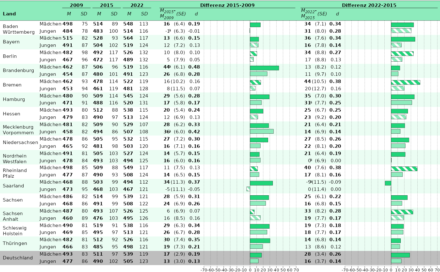
Our goal is to build Abbildung
6.6. Let’s take hoeren for our prototype:
str(dispar$hoeren)
#> List of 4
#>  $ plain      :'data.frame': 2331 obs. of  17 variables:
#>   ..$ label1       : chr [1:2331] "trend (2015 - 2009) for BadenWuerttemberg_maennlich" "trend (2015 - 2009) for crossDiff (BadenWuerttemberg_maennlich - BadenWuerttemberg_total) " "trend (2015 - 2009) of groupDiff (maennlich - weiblich) in TR_BUNDESLAND=BadenWuerttemberg" "trend (2015 - 2009) for BadenWuerttemberg_total" ...
#>   ..$ label2       : chr [1:2331] "year=2015 - year=2009: TR_BUNDESLAND=BadenWuerttemberg, Kgender=maennlich" "[year=2015: (TR_BUNDESLAND=BadenWuerttemberg, Kgender=maennlich)] - [year=2009: (TR_BUNDESLAND=BadenWuerttember"| __truncated__ "[year=2015: (TR_BUNDESLAND=BadenWuerttemberg, Kgender=maennlich) - (TR_BUNDESLAND=BadenWuerttemberg, Kgender=we"| __truncated__ "year=2015 - year=2009: TR_BUNDESLAND=BadenWuerttemberg, Kgender=total" ...
#>   ..$ unit_1       : chr [1:2331] "group_31" "comp_757" "comp_154" "group_202" ...
#>   ..$ unit_2       : chr [1:2331] "group_225" "comp_1373" "comp_307" "group_339" ...
#>   ..$ depVar       : chr [1:2331] "bista" "bista" "bista" "bista" ...
#>   ..$ modus        : chr [1:2331] "JK2.mean__BIFIEsurvey" "JK2.mean__BIFIEsurvey" "JK2.mean__BIFIEsurvey" "JK2.mean__BIFIEsurvey" ...
#>   ..$ parameter    : chr [1:2331] "mean" "mean" "mean" "mean" ...
#>   ..$ comparison   : chr [1:2331] "trend" "trend_crossDiff" "trend_groupDiff" "trend" ...
#>   ..$ TR_BUNDESLAND: chr [1:2331] "BadenWuerttemberg" "BadenWuerttemberg" "BadenWuerttemberg" "BadenWuerttemberg" ...
#>   ..$ Kgender      : chr [1:2331] "maennlich" "maennlich - total" "maennlich - weiblich" "total" ...
#>   ..$ year         : chr [1:2331] "2015 - 2009" "2015 - 2009" "2015 - 2009" "2015 - 2009" ...
#>   ..$ id           : chr [1:2331] "comp_32" "comp_758" "comp_155" "comp_203" ...
#>   ..$ kb           : chr [1:2331] "hoeren" "hoeren" "hoeren" "hoeren" ...
#>   ..$ est          : num [1:2331] -40.74 -6.47 12.97 -34.27 -27.77 ...
#>   ..$ se           : num [1:2331] 7.66 9.42 8.18 6.15 6.71 ...
#>   ..$ p            : num [1:2331] 0 0.492 0.113 0 0 0.453 0.004 0 0.605 0.001 ...
#>   ..$ es           : num [1:2331] -0.395 NA NA -0.336 -0.282 NA NA NA NA NA ...
#>  $ comparisons:'data.frame': 1719 obs. of  4 variables:
#>   ..$ id        : chr [1:1719] "comp_32" "comp_758" "comp_155" "comp_203" ...
#>   ..$ unit_1    : chr [1:1719] "group_31" "comp_757" "comp_154" "group_202" ...
#>   ..$ unit_2    : chr [1:1719] "group_225" "comp_1373" "comp_307" "group_339" ...
#>   ..$ comparison: chr [1:1719] "trend" "trend_crossDiff" "trend_groupDiff" "trend" ...
#>  $ group      :'data.frame': 153 obs. of  5 variables:
#>   ..$ id           : chr [1:153] "group_31" "group_202" "group_85" "group_34" ...
#>   ..$ TR_BUNDESLAND: chr [1:153] "BadenWuerttemberg" "BadenWuerttemberg" "BadenWuerttemberg" "Bayern" ...
#>   ..$ Kgender      : chr [1:153] "maennlich" "total" "weiblich" "maennlich" ...
#>   ..$ year         : chr [1:153] "2009" "2009" "2009" "2009" ...
#>   ..$ kb           : chr [1:153] "hoeren" "hoeren" "hoeren" "hoeren" ...
#>  $ estimate   :'data.frame': 2331 obs. of  7 variables:
#>   ..$ id       : chr [1:2331] "comp_32" "comp_758" "comp_155" "comp_203" ...
#>   ..$ depVar   : chr [1:2331] "bista" "bista" "bista" "bista" ...
#>   ..$ parameter: chr [1:2331] "mean" "mean" "mean" "mean" ...
#>   ..$ est      : num [1:2331] -40.74 -6.47 12.97 -34.27 -27.77 ...
#>   ..$ se       : num [1:2331] 7.66 9.42 8.18 6.15 6.71 ...
#>   ..$ p        : num [1:2331] 0 0.492 0.113 0 0 0.453 0.004 0 0.605 0.001 ...
#>   ..$ es       : num [1:2331] -0.395 NA NA -0.336 -0.282 NA NA NA NA NA ...
#>  - attr(*, "class")= chr [1:2] "list" "report2"
First, I need to search for an appropriate template on this website.
Luckily, we already have a template for Abbildung
6.6. So ewe only need to follow it!
To do this, I first have to look up how my subgroup variable is called.
I can find this out easiest by looking at the group or the
plain data.frame:
str(dispar$hoeren$group)
#> 'data.frame':    153 obs. of  5 variables:
#>  $ id           : chr  "group_31" "group_202" "group_85" "group_34" ...
#>  $ TR_BUNDESLAND: chr  "BadenWuerttemberg" "BadenWuerttemberg" "BadenWuerttemberg" "Bayern" ...
#>  $ Kgender      : chr  "maennlich" "total" "weiblich" "maennlich" ...
#>  $ year         : chr  "2009" "2009" "2009" "2009" ...
#>  $ kb           : chr  "hoeren" "hoeren" "hoeren" "hoeren" ...
My subgroup variable is called Kgender. Now I can use
the prep_tablebarplot() function to prepare the data for
plotting. Of course I have to put my own data into this function:
dat_6.6 <- prep_tablebarplot(
  dispar$hoeren, ## My data.frame
  subgroup_var = "Kgender", ## The subgroup variable
  parameter = c("mean", "sd") ## We need both mean and sd for the plot
)
This is our prepared data.
Data wrangling
For this specific plot, we also have to do some additional (but simple) data transformation, because the data will be plotted in the same order, as we give it into the function. First of all, we can subset the subgroup variable to only extract the groups, we want to use in the plot:
In this BT, the girls should always be on top. To achieve this, we have to sort our data:
gender_hoeren <- gender_hoeren[order(gender_hoeren$subgroup_var, decreasing = TRUE), ]
gender_hoeren <- gender_hoeren[order(gender_hoeren$state_var), ]
Also, we only want to write the Bundesland into the plot every second row, so let’s remove duplicates:
gender_hoeren$state_var[duplicated(gender_hoeren$state_var)] <- " "We can use the process_bundesland() function to add
dashes and replace umlauts. We also want to break the Bundesländer
names, if they are too long, so we set
linebreak = TRUE:
gender_hoeren$state_var <- process_bundesland(gender_hoeren$state_var, linebreak = TRUE)Finally, we have to rename the groups to “Jungen” and “Mädchen” and add an empty column, which will be used as a separator later on:
gender_hoeren$subgroup_var <- gsub("maennlich", "Jungen", gender_hoeren$subgroup_var)
gender_hoeren$subgroup_var <- gsub("weiblich", "Mädchen", gender_hoeren$subgroup_var)

gender_hoeren$empty <- ""
That’s it. The data now has the correct format for plotting.
Plotting
Because we want to plot two plots next to each other, we need to set the column widths of both plots to be the same:
column_widths_stand <- standardize_column_width(
  column_widths = list(
    p1 = c(0.085, 0.05, rep(0.035, 6), 0.015, rep(0.035, 3), NA),
    p2 = c(rep(0.035, 3), NA)
  ),
  plot_ranges = c(142, 142) # Ranges of the x-axes of both plots set in 'axis_x_lims'.
)
To build the tables, we only copy paste from the template on the website:
p_1 <- plot_tablebarplot(
  dat = gender_hoeren,
  bar_est = "est_mean_comp_trend_sameFacet_sameSubgroup_2009_2015",
  bar_label = NULL,
  bar_sig = "sig_mean_comp_trend_sameFacet_sameSubgroup_2009_2015",
  bar_fill = "subgroup_var",
  column_spanners = list(
    "**2009**" = c(3, 4),
    "**2015**" = c(5, 6),
    "**2022**" = c(7, 8),
    "**Differenz 2015-2009**" = c(10, 13)
  ),
  columns_table_se = list(NULL, NULL, NULL, NULL, NULL, NULL, NULL, NULL, NULL, NULL, "se_mean_comp_trend_sameFacet_sameSubgroup_2009_2015", NULL),
  headers = list("**Land**", " ", "*M*", "*SD*", "*M*", "*SD*", "*M*", "*SD*", "", "*M<sub>2015</sub>-<br>M<sub>2009</sub>* ", "*(SE)*", "*d*", " "),
  columns_table = c("state_var", "subgroup_var", "est_mean_comp_none_2009", "est_sd_comp_none_2009", "est_mean_comp_none_2015", "est_sd_comp_none_2015", "est_mean_comp_none_2022", "est_sd_comp_none_2022", "empty", "est_mean_comp_trend_sameFacet_sameSubgroup_2009_2015", "se_mean_comp_trend_sameFacet_sameSubgroup_2009_2015", "es_mean_comp_trend_sameFacet_sameSubgroup_2009_2015"),
  columns_table_sig_bold = list(
    NULL, NULL, "sig_mean_comp_none_2009",
    NULL, "sig_mean_comp_none_2015", NULL, "sig_mean_comp_none_2022", NULL, NULL, "sig_mean_comp_trend_sameFacet_sameSubgroup_2009_2015", NULL, "sig_mean_comp_trend_sameFacet_sameSubgroup_2009_2015"
  ),
  columns_table_sig_superscript = list(NULL, NULL, NULL, NULL, NULL, NULL, NULL, NULL, NULL, "sig_mean_comp_trend_crossDiff_totalFacet_sameSubgroup_2009_2015", NULL, NULL),
  y_axis = "y_axis",
  columns_round = c(rep(0, 11), 2),
  plot_settings = plotsettings_tablebarplot(
    bar_pattern_spacing = 0.0159,
    columns_alignment = c(0, 0, rep(2, 10)),
    columns_width = column_widths_stand$p1, ## This is the column-width object we set above
    columns_nudge_y = c(-0.5, rep(0, 11)),
    headers_alignment = c(0, 0, rep(0.5, 7), 0, 0.5, 0.5, 0),
    headers_row_height = 1.75,
    headers_nudge_x = c(rep(0, 9), 2, rep(0, 3)),
    default_list = abb_6.6
  )
)


p_2 <- plot_tablebarplot(
  dat = gender_hoeren,
  bar_est = "est_mean_comp_trend_sameFacet_sameSubgroup_2015_2022",
  bar_label = NULL,
  bar_sig = "sig_mean_comp_trend_sameFacet_sameSubgroup_2009_2015",
  bar_fill = "subgroup_var",
  column_spanners = list(
    "**Differenz 2022-2015**" = c(1, 4)
  ),
  headers = list(
    "*M<sub>2022</sub>-<br>M<sub>2015</sub>* ",
    "*(SE)*",
    "*d*",
    " "
  ),
  columns_table = c(
    "est_mean_comp_trend_sameFacet_sameSubgroup_2015_2022",
    "se_mean_comp_trend_sameFacet_sameSubgroup_2015_2022",
    "es_mean_comp_trend_sameFacet_sameSubgroup_2015_2022"
  ),
  columns_table_se = list(NULL, "se_mean_comp_trend_sameFacet_sameSubgroup_2015_2022", NULL),
  columns_table_sig_bold = list("sig_mean_comp_trend_sameFacet_sameSubgroup_2015_2022", NULL, "sig_mean_comp_trend_sameFacet_sameSubgroup_2015_2022"),
  columns_table_sig_superscript = list("sig_mean_comp_trend_crossDiff_totalFacet_sameSubgroup_2015_2022", NULL, NULL),
  y_axis = "y_axis",
  columns_round = c(0, 0, 2),
  plot_settings = plotsettings_tablebarplot(
    bar_pattern_spacing = 0.0341,
    columns_alignment = c(2, 2, 2),
    columns_width = column_widths_stand$p2, ## This is the column-width object we set above
    headers_nudge_x = c(2, 0, 0, 0),
    headers_alignment = c(0, 0.5, 0.5, 0),
    headers_row_height = 1.75,
    default_list = abb_6.6
  )
)
Finally, we can combine the plots:
tableplot_6.6 <- combine_plots(list(p_1, p_2))2. Adjustments
Now we can fine/tune the plot, like setting the column widths, nudge
the headers into the right position, etc. You have to look at the plot
in the right format so the changes are shown in the correct proportions.
Either save them as PDF, or use the ggview package:
p <- tableplot_6.6 +
  ggview::canvas(
    235, 130,
    units = "mm"
  )
p
(You have to re-evaluate the plot without the canvas()
function before saving it though.)
If everything is satisfactory, we can save the plot.
save_plot(tableplot_6.6, filename = "C:/Users/hafiznij/Downloads/abb_6.6.pdf", width = 235, height = 130, scaling = 1)3. Put it into a function
As soon as the plot basis works, we can put the code into a dedicated function, to pack it away:
## Data Prep
prepare_6.6_data <- function(dat_kb) {
  dat_6.6 <- prep_tablebarplot(
    dat_kb,
    subgroup_var = "Kgender",
    parameter = c("mean", "sd") ## We need both mean and sd for the plot
  )


  ## Jetzt müssen wir die Daten noch ein wenig für unseren spezifischen Plot umformen
  ## Wir wollen nur männlich und weiblich plotten:
  dat_6.6 <- subset(dat_6.6, subgroup_var %in% c("maennlich", "weiblich"))

  ## Mädchen sollen nach oben, d.h. wir sortieren zuerst absteigend alphabetisch, und dann nach den Bundesländern, um diese wieder in die richtige Reihenfolge zu bekommen
  dat_6.6 <- dat_6.6[order(dat_6.6$subgroup_var, decreasing = TRUE), ]
  dat_6.6 <- dat_6.6[order(dat_6.6$state_var), ]

  ## Dann soll nur in jeder zweiten Zeile das Bundesland geplotted werden, wir entfernen also Duplikate:
  dat_6.6$state_var[duplicated(dat_6.6$state_var)] <- " "

  ## Mit process_bundesland() können wir Bindestriche einfügen und Umlaute austauschen.
  ## linebreak = TRUE damit Bundesländer die aus zwei Wörten bestehen umgebrochen werden
  dat_6.6$state_var <- process_bundesland(dat_6.6$state_var, linebreak = TRUE)

  ## Dann müssen wir noch die Gruppen in Jungen und Mädchen umbenennen
  dat_6.6$subgroup_var <- gsub("maennlich", "Jungen", dat_6.6$subgroup_var)
  dat_6.6$subgroup_var <- gsub("weiblich", "Mädchen", dat_6.6$subgroup_var)

  ## Und eine leere Spalte erzeugen, die später als Trenner dient
  dat_6.6$empty <- ""

  return(dat_6.6)
}

## Plotting
plot_6.6 <- function(dat_prepped) {
  column_widths_stand <- standardize_column_width(
    column_widths = list(
      p1 = c(0.085, 0.05, rep(0.035, 6), 0.015, rep(0.035, 3), NA),
      p2 = c(rep(0.035, 3), NA)
    ),
    plot_ranges = c(140, 142) # Ranges of the x-axes of both plots set in 'axis_x_lims'.
  )


  ## 3. Tabellen erzeugen:
  ## Dafür copy-pasten wir einfach von der Vorlage:

  p_1 <- plot_tablebarplot(
    dat = dat_prepped,
    bar_est = "est_mean_comp_trend_sameFacet_sameSubgroup_2009_2015",
    bar_label = NULL,
    bar_sig = "sig_mean_comp_trend_sameFacet_sameSubgroup_2009_2015",
    bar_fill = "subgroup_var",
    column_spanners = list(
      "**2009**" = c(3, 4),
      "**2015**" = c(5, 6),
      "**2022**" = c(7, 8),
      "**Differenz 2015-2009**" = c(10, 13)
    ),
    columns_table_se = list(NULL, NULL, NULL, NULL, NULL, NULL, NULL, NULL, NULL, NULL, "se_mean_comp_trend_sameFacet_sameSubgroup_2009_2015", NULL),
    headers = list("**Land**", " ", "*M*", "*SD*", "*M*", "*SD*", "*M*", "*SD*", "", "*M<sub>2015</sub>-<br>M<sub>2009</sub>* ", "*(SE)*", "*d*", " "),
    columns_table = c("state_var", "subgroup_var", "est_mean_comp_none_2009", "est_sd_comp_none_2009", "est_mean_comp_none_2015", "est_sd_comp_none_2015", "est_mean_comp_none_2022", "est_sd_comp_none_2022", "empty", "est_mean_comp_trend_sameFacet_sameSubgroup_2009_2015", "se_mean_comp_trend_sameFacet_sameSubgroup_2009_2015", "es_mean_comp_trend_sameFacet_sameSubgroup_2009_2015"),
    columns_table_sig_bold = list(
      NULL, NULL, "sig_mean_comp_none_2009",
      NULL, "sig_mean_comp_none_2015", NULL, "sig_mean_comp_none_2022", NULL, NULL, "sig_mean_comp_trend_sameFacet_sameSubgroup_2009_2015", NULL, "sig_mean_comp_trend_sameFacet_sameSubgroup_2009_2015"
    ),
    columns_table_sig_superscript = list(NULL, NULL, NULL, NULL, NULL, NULL, NULL, NULL, NULL, "sig_mean_comp_trend_crossDiff_totalFacet_sameSubgroup_2009_2015", NULL, NULL),
    y_axis = "y_axis",
    columns_round = c(rep(0, 11), 2),
    plot_settings = plotsettings_tablebarplot(
      axis_x_lims = c(-70, 70),
      bar_pattern_spacing = 0.016,
      columns_alignment = c(0, 0, rep(2, 10)),
      columns_width = column_widths_stand$p1, ## This is the column-width object we set above
      columns_table_sig_superscript_letter = "a",
      columns_table_sig_superscript_letter_nudge_x = 5.5,
      columns_nudge_y = c(-0.5, rep(0, 11)),
      headers_alignment = c(0, 0, rep(0.5, 7), 0, 0.5, 0.5, 0),
      headers_row_height = 1.75,
      headers_nudge_x = c(rep(0, 9), 2, rep(0, 3)),
      default_list = abb_6.6
    )
  )


  p_2 <- plot_tablebarplot(
    dat = dat_prepped,
    bar_est = "est_mean_comp_trend_sameFacet_sameSubgroup_2015_2022",
    bar_label = NULL,
    bar_sig = "sig_mean_comp_trend_sameFacet_sameSubgroup_2015_2022",
    bar_fill = "subgroup_var",
    column_spanners = list(
      "**Differenz 2022-2015**" = c(1, 4)
    ),
    headers = list(
      "*M<sub>2022</sub>-<br>M<sub>2015</sub>* ",
      "*(SE)*",
      "*d*",
      " "
    ),
    columns_table = c(
      "est_mean_comp_trend_sameFacet_sameSubgroup_2015_2022",
      "se_mean_comp_trend_sameFacet_sameSubgroup_2015_2022",
      "es_mean_comp_trend_sameFacet_sameSubgroup_2015_2022"
    ),
    columns_table_se = list(NULL, "se_mean_comp_trend_sameFacet_sameSubgroup_2015_2022", NULL),
    columns_table_sig_bold = list("sig_mean_comp_trend_sameFacet_sameSubgroup_2015_2022", NULL, "sig_mean_comp_trend_sameFacet_sameSubgroup_2015_2022"),
    columns_table_sig_superscript = list("sig_mean_comp_trend_crossDiff_totalFacet_sameSubgroup_2015_2022", NULL, NULL),
    y_axis = "y_axis",
    columns_round = c(0, 0, 2),
    plot_settings = plotsettings_tablebarplot(
      axis_x_lims = c(-70, 72),
      bar_pattern_spacing = 0.034,
      columns_alignment = c(2, 2, 2),
      columns_width = column_widths_stand$p2, ## This is the column-width object we set above
      columns_table_sig_superscript_letter = "a",
      columns_table_sig_superscript_letter_nudge_x = 5.5,
      headers_nudge_x = c(2, 0, 0, 0),
      headers_alignment = c(0, 0.5, 0.5, 0),
      headers_row_height = 1.75,
      default_list = abb_6.6
    )
  )

  tableplot_6.6 <- combine_plots(list(p_1, p_2))

  save_plot(tableplot_6.6,
    filename = paste0(
      "C:/Users/hafiznij/Downloads/abb_6.6_",
      unique(dat_prepped$kb),
      ".pdf"
    ),
    width = 235,
    height = 130,
    scaling = 1
  )

  return(tableplot_6.6)
}
These function now do the same thing we have done above, but we can easily exchange the data set:
prepped_hoeren <- prepare_6.6_data(kap_06$hoeren)
plot_hoeren <- plot_6.6(prepped_hoeren)